11. Gaussian Process Regression & Bayesian Optimization

11.1 Creating a Project #

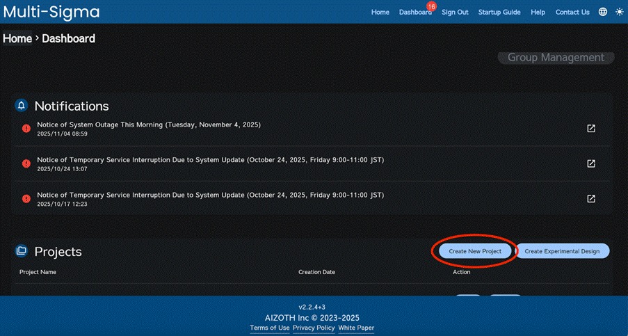
Please note that Gaussian process regression task can be added to the existing project. If you need to create a new project, go to the dashboard, in the Projects section, click “Create New Project” on the right.

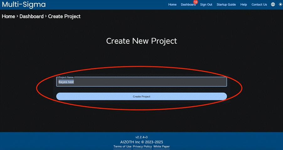
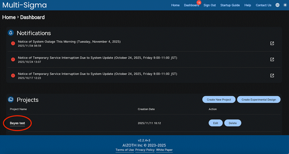
After entering the project name, click “Create Project.” On the dashboard, confirm that the project has been created.

Please click the name of the project you created.

11.2. Creating a Task and Uploading Data #

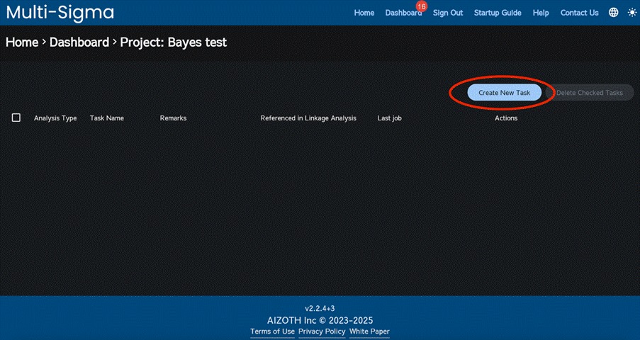
Upon selecting the created project, proceed by clicking on the “Create New Task” button. In the task creation screen, please furnish a task name that effectively represents the specific analysis work you intend to undertake.

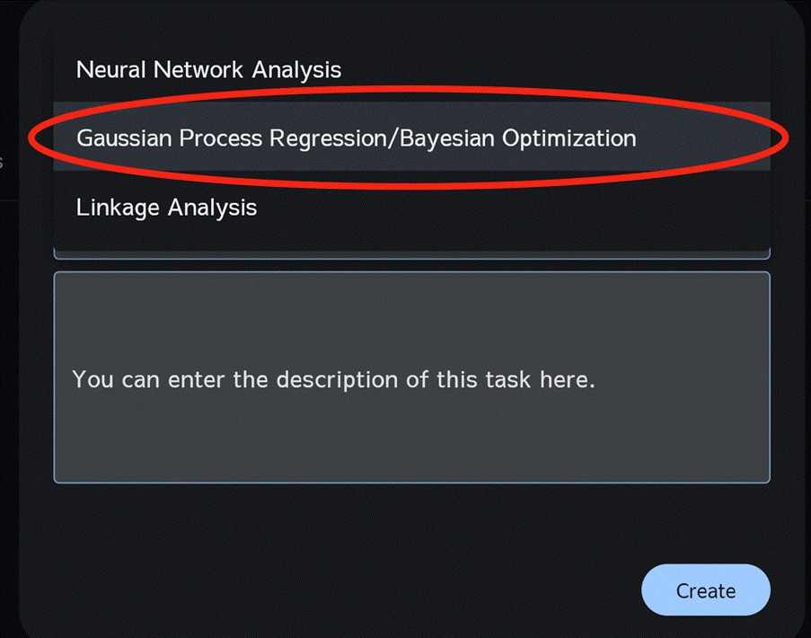
After selecting Gaussian Process Regression & Bayesian Optimization as the analysis method, enter a task name and click “Create”.

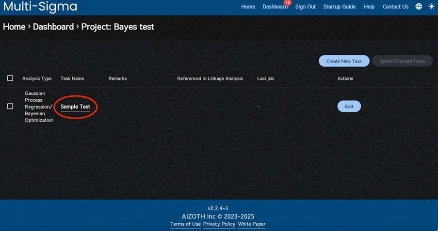
Please click the name of the newly created task.

After clicking the task name, upload the input and output files, then click “Save.”

Both the input and output files must include a header row with the column names. Column names may use alphanumeric characters followed by space, hyphen, or numbers. If the first character contains symbols, spaces or numbers, or if a name consists solely of numbers, an error will occur.

11.3 Transforming Data #

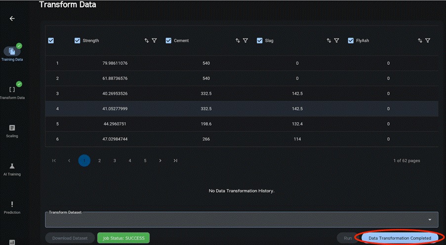
If the dataset contains missing values (e.g., blanks), these may be imputed. If imputation is not required, click Data Transformation Completed to complete data processing.

If the dataset contains missing values and data processing is required, select a transformation method for each variable and impute the missing entries.

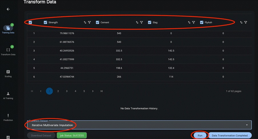
Select the column data (checkbox) to be processed.

Use the leftmost checkbox to select or deselect all.

Select a transformation method and click Run.

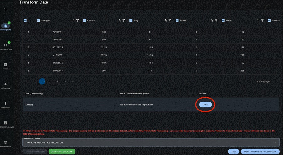
When transformation completes successfully, the transformation history is shown in the order applied.

Click “Undo” for any entry in the history to restore the dataset to its state at that step.

When data processing is complete, click Data Transformation Completed.

Note

If all values in any column are blank, Inf, or NaN, they are automatically imputed to 0.

11.4. Scaling Data #

On the AI Learning screen, please choose the appropriate scaling method (e.g., Min-Max) for each variable, and then proceed by clicking the “Finalize Scaling” button. If you have already performed data preprocessing independently, please select “None”. To revert the data back to it’s original state, press the “Return to Transform Data” and then complete the appropriate scaling method.

If you want to explore an alternative preprocessing method, we recommend creating a new task. It is also advisable to apply the same preprocessing method consistently to each variable. Specifically, for multiple target variables, the Min-Max method is recommended.

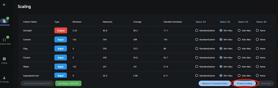
Should the data consist entirely of zeros or the same numeric value, the preprocessing methods “None” and “Abs-Max” will be automatically applied, and it will not be possible to modify them. This precautionary measure is in place to prevent preprocessing errors, so please utilize them as they are.

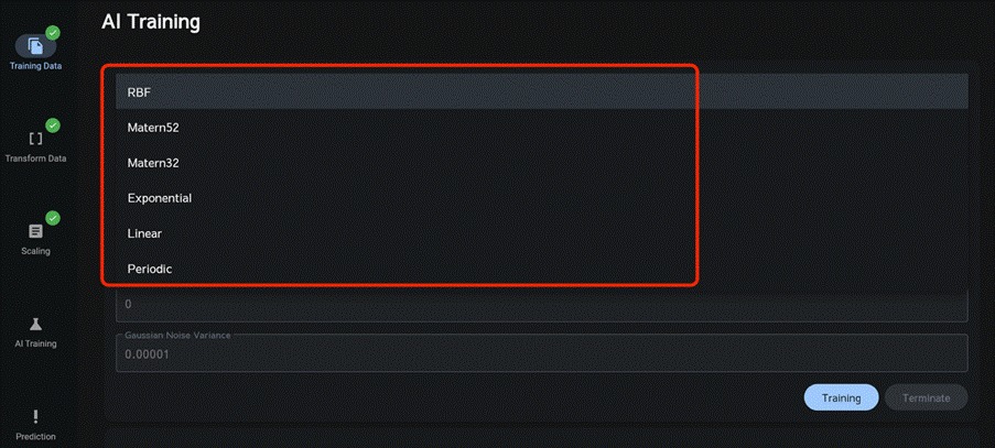
11.5. AI Learning #

On the same AI Learning screen, please proceed by selecting a kernel and clicking the “Training” button. Once the AI learning process has concluded, you can anticipate the appearance of the AI Prediction screen at the bottom of the page. (Note: In Gaussian Process Regression & Bayesian Optimization, the detailed training-results screen shown in Neural Network Analysis is not displayed.)

Please note that this may require a few minutes to complete, so please be patient during this process.

11.6. AI Prediction #

On the AI Prediction screen, please select your preferred prediction model, upload a CSV file that contains a list of unknown independent variables as the input file, and then click “Save” followed by “Predict”. This will enable you to download the predicted values for the target variables based on the provided list of independent variables.

Please note that the input file you use for AI prediction should have a header row with the same column names as the input file used during AI training.

If you later obtain actual results for the predicted values, you can upload them as a validation file. This will allow you to calculate the error between the predictions and the actual results.

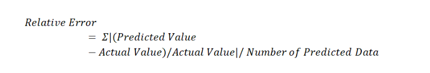
The error is calculated using the following relative error formula. Therefore, when the actual value is close to zero, the model’s prediction will also be close to zero, but even a small absolute difference can result in a very large relative error.

Additionally, clicking “Download Results” will download the relative error, root mean square error (RMSE), and correlation coefficient.

If the prediction results are binary, the ROC curve is available for download. Click “Download ROC” to download it. (If the prediction results are not binary, the button will not be displayed.)

11.7 Contribution Analysis #

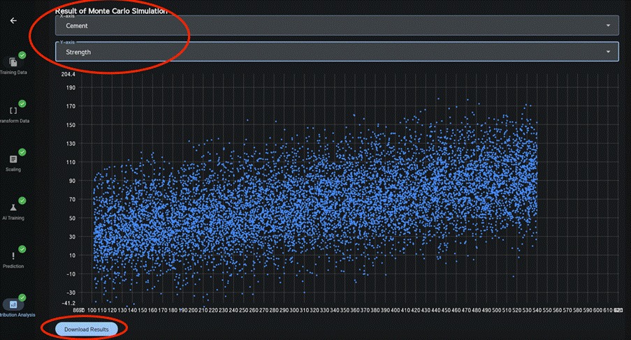
On the Contribution Analysis section, choose whether to enable “Run Monte Carlo Simulation” simultaneously, then click “Run”. The contribution analysis results will be displayed.

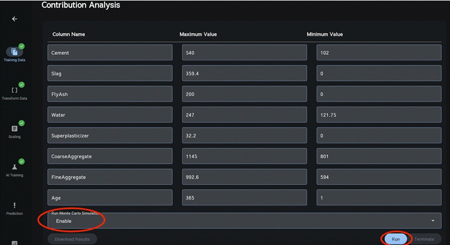
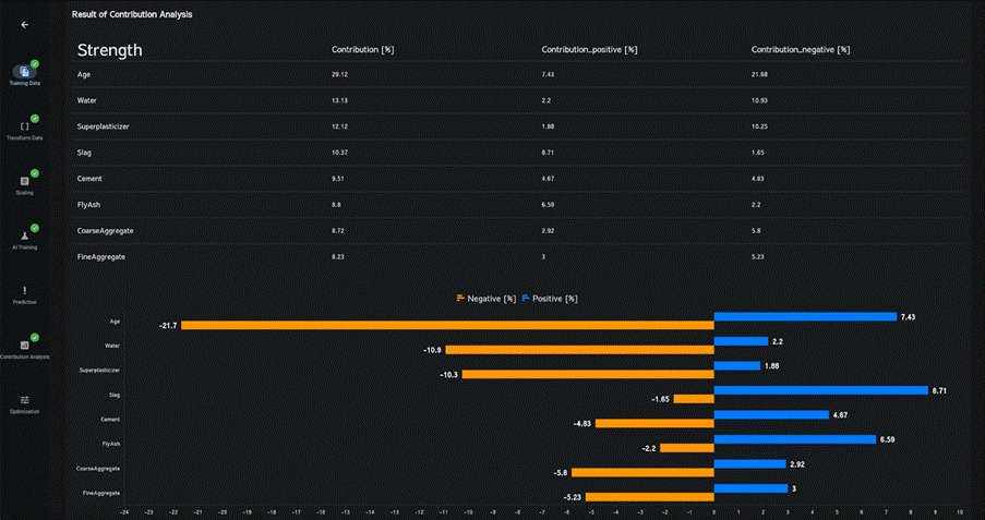
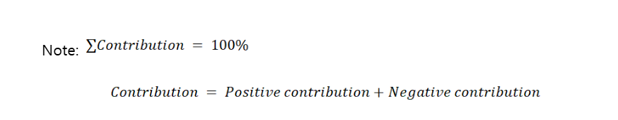
In these results, you’ll find the Contribution values, which show how each independent variable impacts each target variable. Additionally, there are two specific contributions: Positive contribution and Negative contribution, which indicate the positive and negative influences of each independent variable on each target variable. Keep in mind that adjusting the range (maximum and minimum values) of the independent variables can alter the extent of their impact.

To display the Monte Carlo simulation results, select the corresponding X and Y axes.

Click “Download Results” to download the Monte Carlo simulation results.

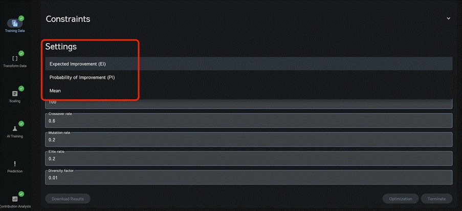
11.8 Optimization #

To perform optimization, please go to the optimization screen and select the search method as either “Expected Improvement,” “Probability of Improvement,” or “Mean”. For each objective variable, choose whether to maximize, minimize, leave uncontrolled, or to set a target value.

11.8.1 Allowing ranges for explanatory variables (inputs) #

If any explanatory variables (inputs) cannot be controlled, select “Uncontrolled” for those variables. The optimization will then be performed for the controlled explanatory variables under the assumption that each uncontrolled explanatory variable can take any value between its minimum and maximum.

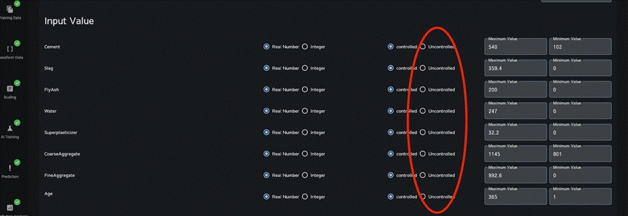
Each row of the optimization-results CSV file also includes the maximum and minimum of each objective, computed under the controlled explanatory-variable settings recorded in that row, when the uncontrolled explanatory variables are allowed to vary from their minimum to their maximum.

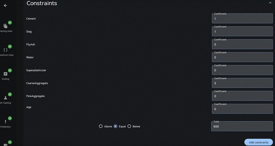
11.8.2 Imposing constraints on explanatory variables (inputs) #

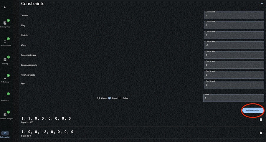
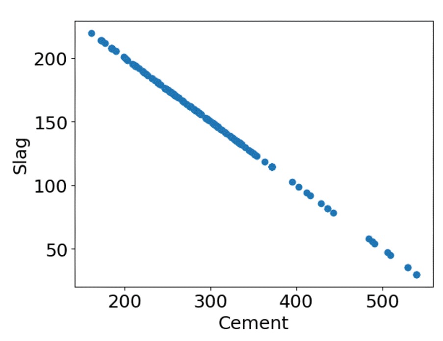
To impose constraints on the explanatory variables, click the section labeled “Constraints”. An input screen like the one below will open; enter the coefficients for each explanatory variable, the total value, and the relation to the total (Above/ Equal / Below). Explanatory variables with a coefficient of 0 are not constrained. The example below applies the constraint Cement × 1 + Slag × 2 = 600.

The figure below shows the downloaded results from running the optimization with constraints set. You can see that the search was conducted under conditions that satisfy those constraints.

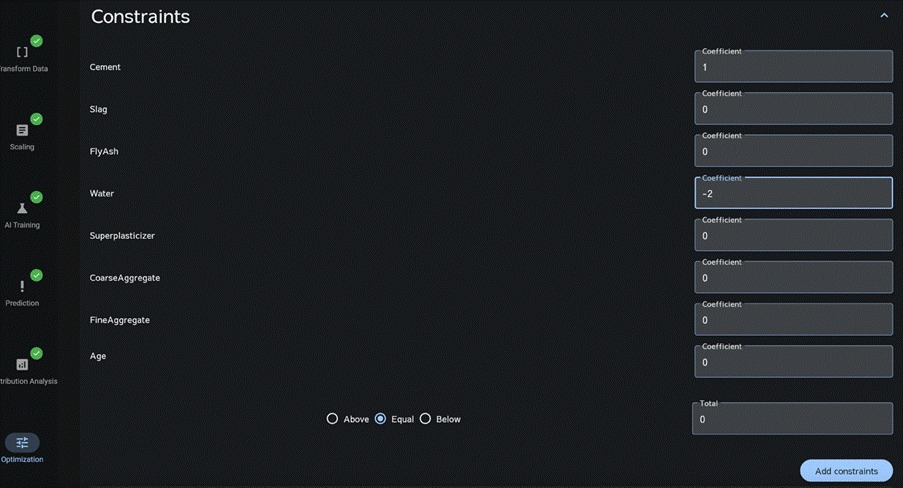
You can also specify negative values for the coefficients and the total.

The figure below shows an example where the constraint Cement × 1 − Water × 2 = 0 is applied.

The figure below shows the downloaded results from running the search with constraints set. You can see that the search was conducted under conditions that satisfy those constraints.

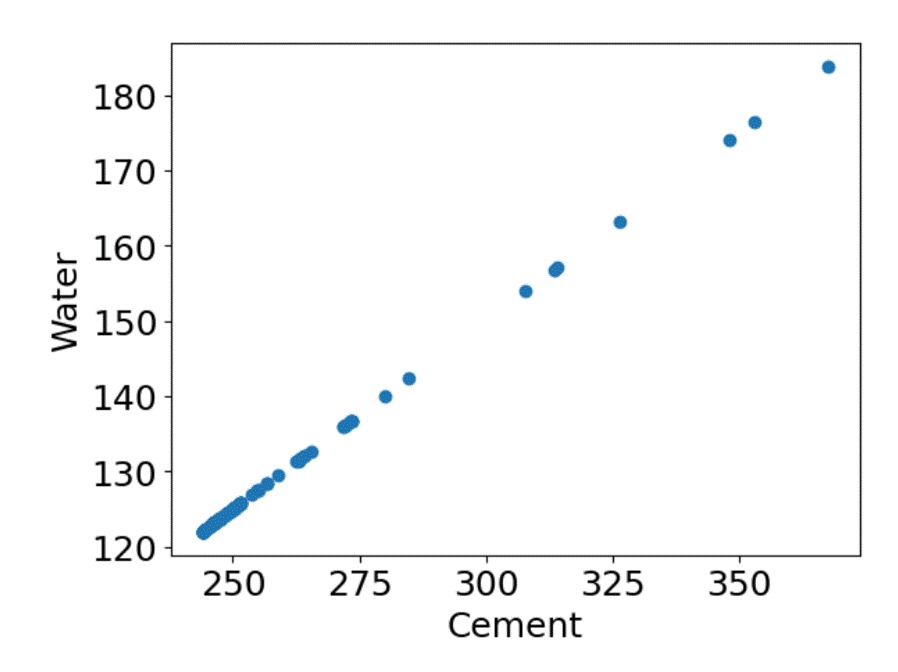
However, note that if negative values are assigned to any coefficients or to the total, or if no feasible solution satisfies the constraints, the results may include outputs that do not meet the constraints.

Multiple constraints can be specified.

After configuring the constraints, click “Add Constraint.”

The constraint settings will be saved.